This document contains a first how-to and usage information for the JAS project.
JAS can be used as any other Java library by adding jas.jar
to the classpath and creating and using objects from JAS classes.
JAS can also be used interactively via the Python Java interpreter
jython (or the Ruby Java interpreter jruby
or the jruby Android App Ruboto-IRB).
This is explained in this page.
For an introduction the API see the API guide.
Since JAS Version 2.2 there is an enhanced interface which allows
direct input of algebraic expressions, see here.
As first example we will discus how to compute a Groebner base with
jython. The jython script will be placed into a file, e.g.
getstart.py.
This script file is executed by calling
jython getstart.py
The script file first imports the desired mathematical classes from the
jas.py script which does all interfacing to the Java library.
For the Epydoc of it see here.
  from jas import Ring
  from jas import Ideal
In our case we need Ring to define an appropriate polynomial ring
and Ideal to define sets of polynomials and have methods to
compute Groebner bases.
Ring takes a string argument which contains required definitions
of the polynomial ring: the type of the coefficient ring, the names of
the used variables and the desired term order.
r = Ring( "Rat(B,S,T,Z,P,W) L" );
The ring definition is stored in the variable r for later use.
The string "Rat(B,S,T,Z,P,W) L" defines the coefficient ring
to be the rational numbers Rat,
the polynomial ring consists of the variables B, S, T, Z, P, W
and the term order L means a lexicographic term order.
For some historical reason the term order orders the variables as
B < S < T < Z < P < W and not the other way.
I.e. the highest or largest variable is always on the left of the list of
variables not on the right as in some other algebra systems.
With
print "Ring: " + str(r);
you can print out the ring definition.
str(r) is the usual python way of producing string representations
of objects, which in our case calls the respective Java method
toString() of the JAS ring object. It produces
Ring: BigRational(B, S, T, Z, P, W) INVLEX
i.e. the coefficients are from the jas class BigRational
and the term order is INVLEX
(INV because the largest variable is on the left).
Next we need to enter the generating polynomials for the ideal.
We do this in two steps, first define a python string with the polynomials
and then the creation of the ideal using the ring definition from before
and the polynomial string.
ps = """
(
 ( 45 P + 35 S - 165 B - 36 ),
 ( 35 P + 40 Z + 25 T - 27 S ),
 ( 15 W + 25 S P + 30 Z - 18 T - 165 B**2 ),
 ( - 9 W + 15 T P + 20 S Z ),
 ( P W + 2 T Z - 11 B**3 ),
 ( 99 W - 11 B S + 3 B**2 ),
 ( B**2 + 33/50 B + 2673/10000 )
)
""";
The polynomial string can be generated by any means python allows for
string manipulation.
In our example we use python multiline strings, which are delimited by
triple quotes """ ... """.
The list of polynomials is delimited by parenthesis ( ... ),
as well as every polynomial is delimited by parenthesis, e.g.
( B**2 + 33/50 B + 2673/10000 ).
The polynomials are separated by commas.
The syntax for polynomials is a sequence of monimals consisting
of coefficients and terms (as products of powers of variables).
The terms can optionally be written with multiplication sign,
i.e. 25 S P can be written 25*S*P.
Variable names must be delimited by white space or some operator,
i.e. you can not write 25 SP because SP
is not a listed variable name in the polynomial ring definition.
Coefficients may not contain white space, i.e. the /
separating the nominator from the denominator may not be surrounded
by spaces, i.e. writing 33 / 50 is not allowed.
Powers of variables can be written with ** or ^,
i.e. the square of B is written as B**2
or B^2.
The ideal is the defined with
f = Ideal( r, ps );
The ideal is contained the the polynomial ring r
and consists of the polynomials from the string ps.
Ideals can be printed with
print "Ideal: " + str(f);
In this example it produces the following output.
Ideal: BigRational(B, S, T, Z, P, W) INVLEX
(
( B^2 + 33/50 B + 2673/10000  ),
( 45 P + 35 S - 165 B - 36  ),
( 35 P + 40 Z + 25 T - 27 S ),
( 15 W + 25 S * P + 30 Z - 18 T - 165 B^2 ),
( -9 W + 15 T * P + 20 S * Z ),
( 99 W - 11 B * S + 3 B^2 ),
( P * W + 2 T * Z - 11 B^3 )
)
The polynomial terms are now sorted with respect to the lexicographical term order. The highest term is first in a polynomial. Also the polynomials are sorted with respect to the term order, but with smallest polynomial first in the list. Finaly we can go to the computation of the Groebner basis of this ideal.
g = f.GB();
The ideal f has a method GB() which
computes the Groebner base. The computed Groebner base is stored
in the variable g which is also an ideal.
It can be printed as the ideal f
print "Groebner base:", g;
The output first shows the output from calling the GB() method
and the the ideal basis.
sequential executed in 136 ms

Groebner base: BigRational(B, S, T, Z, P, W) INVLEX
(
( B^2 + 33/50 B + 2673/10000  ),
( S - 5/2 B - 9/200  ),
( T - 37/15 B + 27/250  ),
( Z + 49/36 B + 1143/2000  ),
( P - 31/18 B - 153/200  ),
( W + 19/120 B + 1323/20000  )
)
I.e. the Groebner base was computed in 135 ms and consists of six polynomials. The polynomials are now monic, i.e. the leading coefficient is 1 and omitted during print out. This concludes the getting started section.
The jython interface to the JAS library consists of the following jython classes. For the Epydoc of them see here.
Ring, Ideal and ParamIdeal
define polynomial rings, ideals and ideals over rings with coefficient parameters.
Ideal has methods for sequential, parallel and distributed
Groebner bases computation, for example
GB(), isGB(),
parGB(), distGB(),
NF() and intersect().
ParamIdeal has methods for comprehensive
Groebner bases computation, for example
CGB(), CGBsystem(), regularGB(),
SolvableRing and SolvableIdeal
define solvable polynomial rings and left, right and two-sided ideals.
SolvableIdeal has methods for left, right and two-sided
Groebner bases computation, e.g.
leftGB(), rightGB(), twosidedGB(),
intersect().
Module and SubModule
define modules over polynomial rings and sub modules.
Module has a method for sequential Groebner bases computation,
e.g. GB().
SolvableModule and SolvableSubModule
define modules over solvable polynomial rings and sub modules.
SolvableModule has methods for left, right and two-sided
Groebner bases computation, e.g.
leftGB(), rightGB(), twosidedGB().
Since JAS Version 2.2 there is an enhanced interface which allows direct input of algebraic expressions. For example the above example looks as follows.
r = Ring( "Z(B,S,T,Z,P,W) L" );
print "Ring: " + str(r);

[B,S,T,Z,P,W] = r.gens();

f1 = 45 * P + 35 * S - 165 * B - 36;
f2 = 35 * P + 40 * Z + 25 * T - 27 * S;
f3 = 15 * W + 25 * S * P + 30 * Z - 18 * T - 165 * B**2;
f4 = - 9 * W + 15 * T * P + 20 * S * Z;
f5 = P * W + 2 * T * Z - 11 * B**3;
f6 = 99 * W - 11 *B * S + 3 * B**2;
f7 = 10000 * B**2 + 6600 * B + 2673;

F = [ f1, f2, f3, f4, f5, f6, f7 ];

I = r.ideal( "", list=F );
The definition of the polynomial ring with
r = Ring( "Z(B,S,T,Z,P,W) L" )
is obligatory as before. As above many coefficient rings,
e.g. Z, and term orders, e.g. L, can be selected.
New is the setup of a list of generators of the polynomial ring with
[B,S,T,Z,P,W] = r.gens(). The sequence of jython variable names
B, S, T, Z, P, W should match the sequence of variables as defined
in the creation of the ring.
A jython variable defined with this idiom then represents a polynomial
of the respective ring in the respectively named variable.
For example B is the polynomial in ring r
in the variable named 'B'.
The so defined polynomial generators can then be used to
build (nearly) arbitrary expressions.
For example the polynomial f5 is defined by the expression
P * W + 2 * T * Z - 11 * B**3.
Since Python (and jython) has no built-in rational number support,
only (arbitrary long) integers can be used as numbers.
As a work around we propose to use python tuples or lists
with 2 entries as rational numbers.
Floating point numbers are truncated to integer.
For exponentiation one must use the double star ** as the
carret ^ has a fixed meaning as as bitwise XOR.
Additionally all operators must explicitly be written,
even between coefficients and variables.
The literal representation of the polynomial expression does not restrict
the definition of the ring. So the polynomial ring can be defined with
rational coefficients but Python integers can be used as operands.
If you need to enter rational numbers you must use
python tuple or list notation (see below)
or explicitly the JAS class BigRational.
Continuing with the example, we build a list of polynomials
with a Python list F = [ f1, f2, f3, f4, f5, f6, f7 ].
Finally the ideal is created as usual with the
ideal method of r as
I = r.ideal( "", list=F ).
When python tuples or lists of integers are used as operands of JAS ring elements
they are interpreted as rational or complex rational numbers.
For example in the construction of Legendre polynomials a
rational number r = 1/n appears.
As tuple literal it is written (1,n) and
as list literal it can be written as [1,n].
p = (2*n-1) * x * P[n-1] - (n-1) * P[n-2];
r = (1,n); # no rational numbers in python, use tuple notation
p = r * p;
In the same way complex rational numbers can be written as nested tuples.
For example 1/n + 1/2 i can be written as
((1,n),(1,2)).
If the second list element is omited it is asumed to be one.
In this case it can however not be written as tuple,
since one nesting level would be removed as expression parenthesis.
If the tuples or lists contain more than 2 elements, the rest is
silently ignored.
For example 1/n as complex number can be written as
[(1,n)] (but not as ((1,n))).
Different nesting levels are allowed, i.e.
((1,n),2) or (0,(1,n)) are legal.
In case the types (nesting levels) of operands do not match,
for example when adding a rational to a complex number
(low level) class cast errors will be thrown.
For example in (1,n) + (0,(1,n)) the exception
edu.jas.arith.BigComplex cannot be cast to edu.jas.arith.BigRational
will be thrown.
Further examples can be found in the jython files
polynomial.py,
legendre.py,
hermite.py or
chebyshev.py.
Besides the computation of Gröbner bases JAS is able to use them to solve various other problems. In this sub-section we present the computation of real roots of systems of (algebraic) equations. When the system of equations has only finitely many real roots, such systems define so called zero dimensional ideals, they can be computed as follows.
r = PolyRing(QQ(),"x,y,z",PolyRing.lex);
print "Ring: " + str(r);
print;

[one,x,y,z] = r.gens();

f1 = (x**2 - 5)*(x**2 - 3)**2;
f2 = y**2 - 3;
f3 = z**3 - x * y;

F = r.ideal( list=[f1,f2,f3] );

R = F.realRoots();
F.realRootsPrint()
In the above example we compute the real roots of the equations
defined by the polynomials f1, f2, f3. First we define
the polynomial ring and then construct the ideal F from
the given polynomials. The method F.realRoots() computes
the real roots and method F.realRootsPrint() prints a
decimal approximation of tuples of real roots. The output of the last
method call looks as follows.
[-1.7320508076809346675872802734375, -1.7320508076809346675872802734375, 1.4422495705075562000274658203125]
[1.7320508076809346675872802734375, 1.7320508076809346675872802734375, 1.4422495705075562000274658203125]

[1.7320508076809346675872802734375, -1.7320508076809346675872802734375, -1.4422495705075562000274658203125]
[-1.7320508076809346675872802734375, 1.7320508076809346675872802734375, -1.4422495705075562000274658203125]

[0.50401716955821029841899871826171875, 2.236067977384664118289947509765625, -1.7320508076809346675872802734375, -1.5704178023152053356170654296875]
[-0.50401716955821029841899871826171875, -2.236067977384664118289947509765625, 1.7320508076809346675872802734375, -1.5704178023152053356170654296875]
[-3.96811878503649495542049407958984375, -2.236067977384664118289947509765625, -1.7320508076809346675872802734375, 1.5704178023152053356170654296875]
[3.96811878503649495542049407958984375, 2.236067977384664118289947509765625, 1.7320508076809346675872802734375, 1.5704178023152053356170654296875]
The roots in the tuples [-1.7320508076809346675872802734375,
-1.7320508076809346675872802734375,
1.4422495705075562000274658203125] correspond to the roots in
the variables [x, y, z]. The last four tuples have four
entries [0.50401716955821029841899871826171875,
2.236067977384664118289947509765625,
-1.7320508076809346675872802734375,
-1.5704178023152053356170654296875], where the first entry
stems from an internal field extension, which was needed to correctly
identify the roots of the ideal and are to be ignored. That is the
tuple [2.236067977384664118289947509765625,
-1.7320508076809346675872802734375,
-1.5704178023152053356170654296875] without the first entry is
a real root of the ideal. That is, the decimal approximation of the
real roots are the following 8 tuples.
[-1.7320508076809346675872802734375, -1.7320508076809346675872802734375, 1.4422495705075562000274658203125] [1.7320508076809346675872802734375, 1.7320508076809346675872802734375, 1.4422495705075562000274658203125] [1.7320508076809346675872802734375, -1.7320508076809346675872802734375, -1.4422495705075562000274658203125] [-1.7320508076809346675872802734375, 1.7320508076809346675872802734375, -1.4422495705075562000274658203125] [2.236067977384664118289947509765625, -1.7320508076809346675872802734375, -1.5704178023152053356170654296875] [-2.236067977384664118289947509765625, 1.7320508076809346675872802734375, -1.5704178023152053356170654296875] [-2.236067977384664118289947509765625, -1.7320508076809346675872802734375, 1.5704178023152053356170654296875] [2.236067977384664118289947509765625, 1.7320508076809346675872802734375, 1.5704178023152053356170654296875]
More details and further examples can be found in the jython file
0dim_real_roots.py.
Univariate power series can be constructed via
the SeriesRing class.
In the following example we create a new power series ring
pr in the variable y over the rational numbers.
The creation of power series is done in the same way as
polynomials are created. There are additional methods like
r.exp() or r.sin() to create the
exponential power series or the power series for the sinus function.
pr = SeriesRing("Q(y)");
print "pr:", pr;

one = pr.one();
r1 = pr.random(4);
r2 = pr.random(4);

print "one:", one;
print "r1:", r1;
print "r2:", r2;

r4 = r1 * r2 + one;
e = pr.exp();
r5 = r1 * r2 + e;

print "e:", e;
print "r4:", r4;
print "r5:", r5;
Once power series are created, for example
r1, r2, e above, it is possible to use
arithmetic operators to built expressions of power series like
'r1 * r2 + one' or 'r1 * r2 + e'.
pr: BigRational((y))

one: 1  + BigO(y^11)
r1:  - 14/3 * y + 3/5 * y^6 + 1/12 * y^8 + 1/7 * y^10 + BigO(y^11)
r2:  - 9/11  - 11/9 * y - 4/3 * y^4 + 7/9 * y^5 + 3 * y^6 - 3/2 * y^8 + BigO(y^11)

e: 1  + 1 * y + 1/2 * y^2 + 1/6 * y^3 + 1/24 * y^4 + 1/120 * y^5 + 1/720 * y^6 + 1/5040 * y^7 + 1/40320 * y^8 + 1/362880 * y^9 + 1/3628800 * y^10 + BigO(y^11)
r4: 1  + 42/11 * y + 154/27 * y^2 + 56/9 * y^5 - 6119/1485 * y^6 - 221/15 * y^7 - 3/44 * y^8 + 745/108 * y^9 - 353/385 * y^10 + BigO(y^11)
r5: 1  + 53/11 * y + 335/54 * y^2 + 1/6 * y^3 + 1/24 * y^4 + 2243/360 * y^5 - 97871/23760 * y^6 - 14851/1008 * y^7 - 30229/443520 * y^8 + 2503201/362880 * y^9 - 36599029/39916800 * y^10 + BigO(y^11)
It is also possible to create power series by defining a generating function or by defining a fixed point with respect to a map between power series.
def g(a):
    return a+a;
ps1 = pr.create(g);

class coeff( Coefficients ):
    def generate(self,i):
        ...
ps6 = pr.create( clazz=coeff( pr.ring.coFac ) );

class cosmap( PowerSeriesMap ):
    def map(self,ps):
        ...
ps8 = pr.fixPoint( cosmap( pr.ring.coFac ) );
More details and further examples can be found in the jython file
powerseries.py.
The jruby interface to the JAS library consists essentially of the same classes as the jython interface, but the ruby language, syntax and semantics is used. For the Rdoc of them see here.
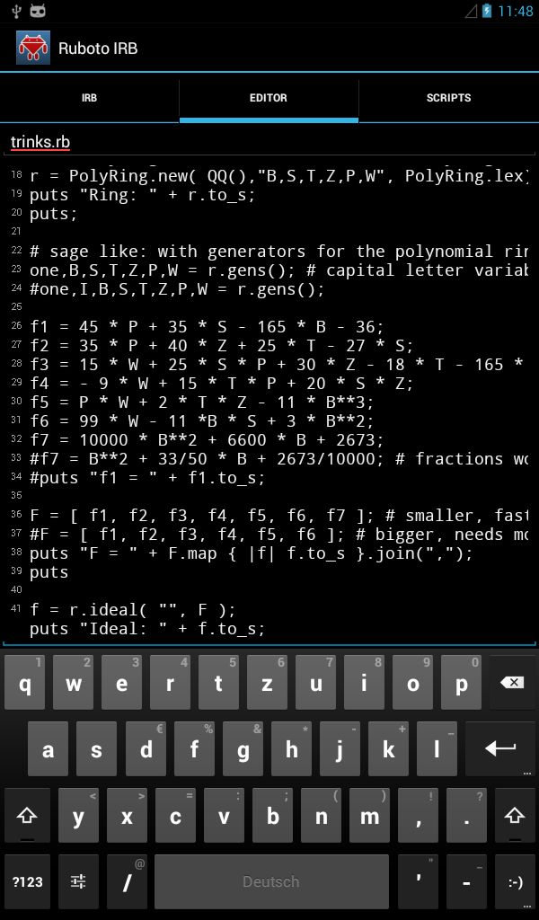
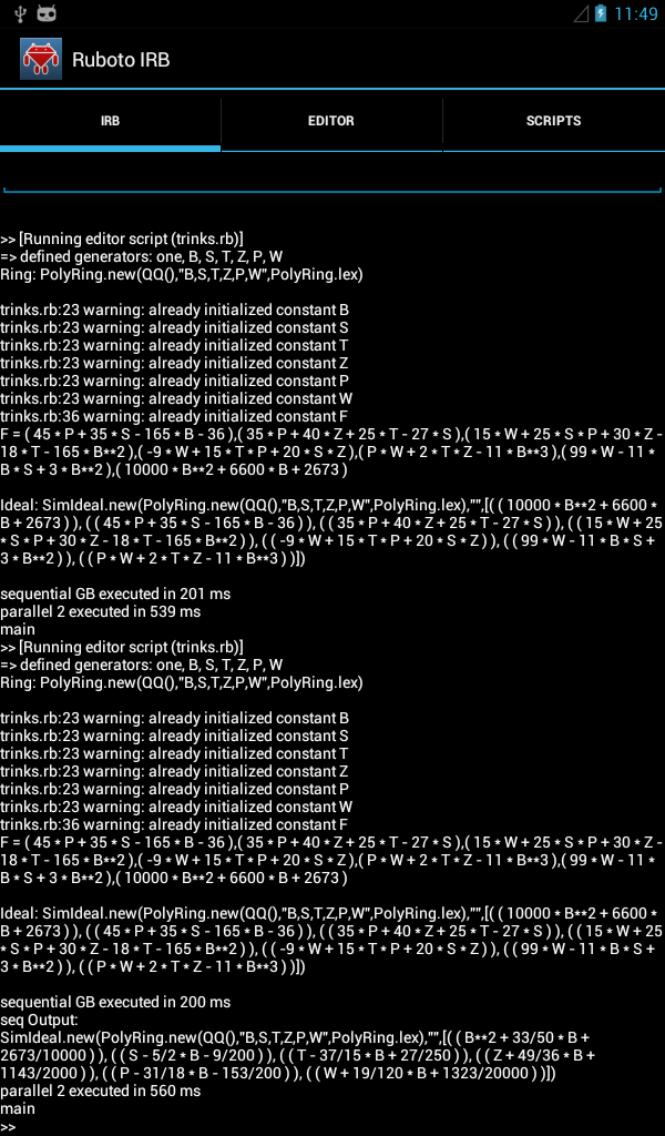
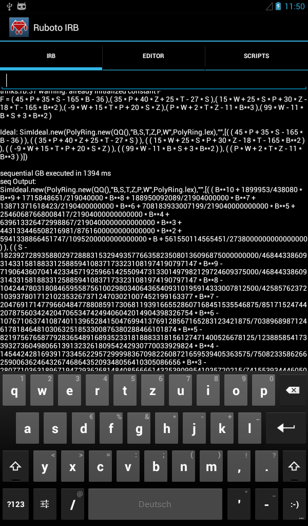
For the Android app the main screen with the "trinks.rb" example and its output looks as follows.
The Trinks example from above looks in Ruby as follows.
require "examples/jas"

r = PolyRing.new( QQ(),"B,S,T,Z,P,W", PolyRing.lex);
puts "Ring: " + r.to_s;
puts;

one,B,S,T,Z,P,W = r.gens();

f1 = 45 * P + 35 * S - 165 * B - 36;
f2 = 35 * P + 40 * Z + 25 * T - 27 * S;
f3 = 15 * W + 25 * S * P + 30 * Z - 18 * T - 165 * B**2;
f4 = - 9 * W + 15 * T * P + 20 * S * Z;
f5 = P * W + 2 * T * Z - 11 * B**3;
f6 = 99 * W - 11 *B * S + 3 * B**2;
f7 = B**2 + 33/50 * B + 2673/10000; # fractions work with ruby

F = [ f1, f2, f3, f4, f5, f6, f7 ]; # smaller, faster
puts "F = " + F.map { |f| f.to_s }.join(",");
puts

f = r.ideal( "", F );
puts "Ideal: " + f.to_s;
puts;

rg = f.GB();
puts "seq Output:", rg;
puts;
The definition of the polynomial ring with
r = PolyRing.new( QQ(),"B,S,T,Z,P,W", PolyRing.lex)
is obligatory as before. As above many coefficient rings,
e.g. QQ, and term orders, e.g. PolyRing.lex, can be selected.
The setup of a list of generators of the polynomial ring is in Ruby
one,B,S,T,Z,P,W = r.gens(). The sequence of jruby variable names
B, S, T, Z, P, W should match the sequence of variables as defined
in the creation of the ring.
A jruby variable defined with this idiom then represents a polynomial
of the respective ring in the respectively named variable.
For example B is the polynomial in ring r
in the variable named 'B'.
The so defined polynomial generators can then be used to
build (nearly) arbitrary expressions.
For example the polynomial f5 is defined by the expression
P * W + 2 * T * Z - 11 * B**3.
Since Ruby (and jruby) has built-in rational number support,
also integer fractions can be used as coefficients.
For exponentiation one uses the double star ** as with Python.
Additionally all operators must explicitly be written,
even between coefficients and variables.
Continuing with the example, we build a list of polynomials
with a Ruby list F = [ f1, f2, f3, f4, f5, f6, f7 ].
Finally the ideal is created as usual with the
ideal method of r as
f = r.ideal( "", F ) in the same way as in Python.
Solvable polynomial rings are non commutative polynomial rings where the non commutativity is expressed by commutator relations. Commutator relations are stored in a data structure called relation table. In the definition of a solvable polynomial ring this relation table must be defined. E.g the definition for the ring of a Weyl algebra is
Rat(a,b,e1,e2,e3) L
RelationTable
(
 ( e3 ), ( e1 ), ( e1 e3 - e1 ),
 ( e3 ), ( e2 ), ( e2 e3 - e2 )
)
The relation table must be build from triples of (commutative) polynomials.
A triple p1, p2, p3 is interpreted as non commutative
multiplication relation p1 .*. p2 = p3.
Currently p1 and p2 must be single term, single variable
polynomials. The term order must be choosen such that
leadingTerm(p1 p2) equals leadingTerm(p3)
and p1 > p2 for each triple.
Polynomial p3 must be in commutative form,
i.e. multiplication operators occuring in it are commutative.
Variables for which there are no commutator relations are assumed to
commute with each other and with all other variables,
e.g. the variables a, b in the example.
Polynomials in the generating set of an ideal are also assumed to be
in commutative form. This will be changed in the future to allow the
multiplication operator to mean non-commutative multiplication.
A complete example is contained in the python script
solvable.py.
Running the script computes a left, right and twosided Groebner base
for the following ideal
(
 ( e1 e3^3 + e2^10 - a ),
 ( e1^3 e2^2 + e3 ),
 ( e3^3 + e3^2 - b )
)
The left Groebner base is
(
 ( a ), ( b ),
 ( e1^3 * e2^2 ), ( e2^10 ), ( e3 )
)
the twosided Groebner base is
(
 ( a ), ( b ), ( e1 ), ( e2 ), ( e3 )
)
and the right Groebner base is
(
 ( a ), ( b ), ( e1 ), ( e2^10 ), ( e3 )
)
A module example is in
armbruster.py
and a solvable module example is in
solvablemodule.py.
Last modified: Sat Dec 1 19:25:47 CET 2012